#Dynamic Programming Pt.1

#Shortest path as network flow

Given undirected graph $G = (V, E)$ , start node $s$ , and end node $t$ , we want to find the shortest path $s ⇝ t$ .

Each edge $ij \in E$ has a non-negative cost $c_{ij}$ . Typically the distance.
The $⇝$ arrow means the path from $s$ to $t$ , including arbitrarily many intermediate vertices.

#Decision Variables

We want to find which edge to take from $E$ .

x_{ij} = {10 if ij is in the shortest path otherwise

#Objective

Minimize the path cost.

min subject to ij \in E \sum c_{ij} x_{ij} ⎩ ⎨ ⎧ \forall v \in V, Flow out - Flow in = ⎩ ⎨ ⎧ 0 - 1 1 if v \neq = s, t if v = s if v = t

We could solve the shortest path problem with a general LP solver, but we have more efficient algorithms.

#Dijkstra’s Algorithm

The following pseudocode is from my own algorithm notes but it does the same thing as what we did in class.

Pseudocode

Complexity

function Initialize(G, start):
	for each vertex v in G:
		dist[v] = Infinity
		pred[v] = nothing
	dist[start] = 0
	pred[start] = nothing
	return dist, pred

function NonNegativeDijkstras(G, start):
	dist, pred = Initialize(G, start)
	dist[start] = 0

	queue = PriorityQueue()
	for each vertex v in G:
		put v in queue with priority dist[v]

	while queue is not empty:
		u = queue.ExtractMin()
		for each adjacent vertex v:
			if dist[v] > dist[u] + weight(uv):
				dist[v] = dist[u] + weight(uv)
				pred[v] = u
				queue.UpdatePriority(v, dist[v])


// matched to each line








O(V)



O(V log V)


O(E) with inner for loop
O(log V) for heaps
already counted



O(log V) for heaps

where queue.ExtractMin() grabs the vertex with the shortest distance.

#Example. In-class practice graph

Source: Canvas, Shortest_path_problem_in_class.pdf — Source: Canvas, `Shortest_path_problem_in_class.pdf`

Running Dijkstra’s algorithm with $start = A$ gives us shortest path from $A$ to every other node:


==> Selected start: A
╭──────────────┬────────────────────────────────┬────────────╮
│ End Vertex   │ path                           │   distance │
├──────────────┼────────────────────────────────┼────────────┤
│ A            │ []                             │          0 │
│ B            │ ['A', 'B']                     │         10 │
│ C            │ ['A', 'B', 'C']                │         39 │
│ D            │ ['A', 'E', 'F', 'G', 'D']      │         48 │
│ E            │ ['A', 'E']                     │          8 │
│ F            │ ['A', 'E', 'F']                │         22 │
│ G            │ ['A', 'E', 'F', 'G']           │         34 │
│ H            │ ['A', 'E', 'F', 'G', 'H']      │         53 │
│ I            │ ['A', 'E', 'I']                │         20 │
│ J            │ ['A', 'E', 'F', 'J']           │         37 │
│ K            │ ['A', 'E', 'F', 'G', 'K']      │         43 │
│ L            │ ['A', 'E', 'F', 'G', 'K', 'L'] │         61 │  <== Path from A to L
╰──────────────┴────────────────────────────────┴────────────╯

#Optimal Substructure

Suppose $s ⇝ t$ is the shortest path from $s$ to $t$ , and $v$ is an intermediate node.

Then the sub-path $s ⇝ v$ and $v ⇝ t$ are both shortest paths from $s$ to $v$ , $v$ to $t$ respectively.

#Asymmetric Traveling Salesman Problem

For a directed graph $G = (V, A)$ , a non-negative cost $c_{ij}$ for each arc $i \to j$ , we want to find the shortest tour (visit all nodes exactly once and return to the starting node)

#Decision Variable

x_{ij} = {10 if i \to j is in the final tour otherwise

#Objective

Minimize the total cost.

min i \to j \in A \sum c_{ij} x_{ij}

#Constraints

For each $v \in V$ , let the set of edges entering $v$ be $δ^{-}$ , edges leaving $v$ be $δ^{+}$ :

δ^{-} (v) = {i \to v \in A} δ^{+} (v) = {v \to i \in A}

We should pass through $v$ exactly once, so 1 edge in 1 edge out.

a \in δ^{-} (v) \sum x_{a} a \in δ^{+} (v) \sum x_{a} = 1 = 1

#Sub-tour elimination

The graph should also be connected, no isolated subgraphs

We don’t want (1) basically, since there’s complete tour. Source

#The Dantzig-Fulkerson-Johnson (DFJ) formulation

\forall S \subset V, S \neq = \emptyset, define δ^{+} (S) = {i \to j \in A : i \in S, j \in / S} a \in δ^{+} (S) \sum x_{a} ⩾ 1

This constraint is what makes TSP an NP-Hard problem, the number of possible $S$ ’s is the size of the power set of $V$ , which is $P (V) = 2^{V}$

#The Miller–Tucker–Zemlin (MTZ) formulation

For each node $i \in V$ , label with $u_{i} \in N$ except the starting node.

{u_{j} > u_{i} no constraints if x_{ij} = 1 if x_{ij} = 0

The idea is we must go to a node that has a larger label than the current node.

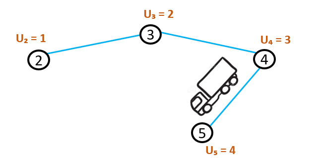
This prevents us from going into cycles, since if we do, we will eventually travel to a node with a smaller label, which violates the constraint.

#Symmetric TSP

Now we consider a undirected graph $G = (V, E)$ , a non-negative cost $c_{ij}$ for each edge $ij$ . We also know that $c_{ij} = c_{ji}$ .

#Objective

Same as the asymmetric case.

min e \in E \sum c_{e} x_{e}

#Constraints

Let $δ (v)$ be the set of edges connected to node $v$ :

δ (v) = {i v \in E}

The one edge in, one edge out constraint is:

\forall v \in V, e \in δ (v) \sum x_{e} = 2

Let $δ (S), S \subset V$ be the set of edges that have one node in $S$ and one node not in $S$ :

δ (S) = {ij : i \in S, j \in / S}

Using the DFJ formulation for sub-tour elimination, we have:

\forall S \subset V, S \neq = \emptyset e \in δ (S) \sum x_{e} ⩾ 2

#Dynamic Programming (DP)

#General formulation

Every DP problem has the following properties:

Stages : $t = 1, 2, \dots, T$

State at stage $t$ : $s_{t}$

Value function : $v_{t} (s_{t})$

Transition cost : $c (s_{t - 1}, s_{t})$

v_{t} (s_{t}) = min / max {v_{t - 1} (s_{t - 1}) + c (s_{t - 1}, s_{t})}

#Theorem. Principle of optimality

If $v_{t} (s_{t})$ is optimal, then all the subproblems $v_{t - 1} (s_{t - 1})$ are also optimal.

#0-1 Knapsack

Given a backpack with capacity $b$ , and $n$ items where each item takes up capacity $a_{i}$ and is worth $c_{i}$ dollars. Decide which items to take.

#Objective

Let $x_{i}$ be the indicator variable of whether to take item $i$ , we want to maximize total profit:

max subject to i = 1 \sum n x_{i} c_{i} ⎩ ⎨ ⎧ i = 1 \sum n x_{i} a_{i} x_{i} < b \in {0, 1}

If we don’t have the integer constraint $x_{i} \in {0, 1}$ , we can just take the items with maximum profit-to-capacity ratio: $\frac{c _{i}}{a _{i}}$ .

#DP Formulation

Stage
: The maximum item index $1, 2, \dots, n$ . If we are in stage $k$ , we only consider items $1, 2, \dots, k$ .

State
: $w$ , remaining capacity of the backpack

Value function : $v_{k} (w)$ , max profit given capacity $w$ and items $1, 2, \dots k$

v_{k} (w) = max {v_{k - 1} (w - a_{k}) + c_{k} v_{k - 1} (w)}

We can try to take item $k$ if it fits, or we can skip $k$ .

#Bounded Knapsack

Now suppose each items has a maximum of $u_{i}$ copies.

0 ⩽ x_{i} ⩽ u_{i}

In this case we include the number of copies as part of the state, $v_{k} (w, s_{k})$ now represents the maximum profit with capacity $w$ , $s_{k}$ copies of item $k$ , and using item $1 \dots k$ .

v_{k} (w, s_{k}) = 0 ⩽ s_{k} ⩽ u_{k} max {v_{k - 1} (w - s_{k} a_{k}) + s_{k} c_{k}}

#Direct TSP with dynamic programming

Consider the graph $G = (V, A)$

i \ j 12345 101535230412315034454201543130

The subproblem is a graph with the sam vertices, but less edges.