# Convex Optimization

\lambda \bold x + (1-\lambda)\bold y \in S

f(\lambda\bold x + (1-\lambda)\bold y)\leqslant \lambda f(\bold{x}) + (1-\lambda)f(\bold{y})

A nice connection shows up of we consider the more general definition of a linear function. f:\R \to\R is linear if it satisfies:

f(\alpha x + \beta y) = \alpha f(x) + \beta f(y)

for constants \alpha, \beta and all x,y in f's domain.

Another definition of a convex function is:

f(\alpha x + \beta y) \leqslant \alpha f(x) + \beta f(y)

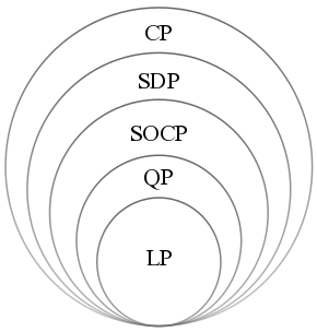
So we can see that linear optimization is just a special case of convex optimization.

Let the domain be (-\infty, \infty),

• f(x) = e^x, f(x) = x^2 are convex

• f(x) = \sqrt{x}, f(x) = x^3 are not convex

A convex optimization program looks like the following:

\begin{aligned}
    \min\quad& f_0(\bold x)\\
    \text{subject to }\quad & \left\{\begin{aligned}&
         \left.\begin{aligned}
        f_1(\bold x)&\leqslant 0\\
        f_2(\bold x)&\leqslant 0\\
        \qquad \vdots\\
        f_m(\bold x)&\leqslant 0
    \end{aligned}\right\}\text{Inequality Constraints}\\\\
    &\left.\begin{aligned}
        h_1(\bold x) &= 0\\
        \qquad \vdots\\
        h_p(\bold x) &= 0
    \end{aligned}\right\}\text{Equality Constraints}
    \end{aligned}
    \right.
\end{aligned}

where f_0\dots f_m: \R^m\to \R are convex, h_1\dots h_p: \R^m\to \R are linear.

Let X be the set of solutions / feasible region:

X = \{\bold{x}\in\R^m\mid \bold{x} \text{ satisfies all the constraints} \}

Linear functions of the form \bold{a^\top x +b} are both convex and concave. LP is a special case of convex optimization

In \R^2, consider the constraints f_1, f_2 \leqslant 0 where:

\begin{aligned}
    f_1(\bold x) &= x_1^2 + x_2^2 - 1\\
    f_2(\bold x) &= e^{x_1} - x_2 - 1
\end{aligned}

We can see that the overlapped region is convex.

Infeasible

X=\varnothing, optimal value = \infty

Unbounded

|X| = \infty, optimal value = -\infty

Optimal

We either have a finite solution or the solution is infinite. For example \min e^{-x}, the optimal value is 0, but we need x\to \infty.

A general cone program has the form:

\begin{aligned}
    \min\quad &\bold c^\top \bold x\\
    \text{subject to}\quad & \|A_i\bold x + \bold b_i\|_2\leqslant \bold c_i^\top \bold x +  d_i\qquad 1\leqslant i\leqslant m
\end{aligned}

where \|\cdot\|_2 is the l_2 norm.

A second order cone has the following form:

\{(\bold x,t)\in\R^2\times \R: \|\bold x\|_2 \leqslant t\}

Linear programming is a special case of SOCP.

\begin{matrix}
    \begin{aligned}
        \min \quad & \bold c^\top  \bold x\\
        \text{subject to}\quad &\begin{aligned}
            A\bold x &= \bold b\\
            \bold x &\geqslant 0
        \end{aligned}
    \end{aligned}

    &\iff
    &
    \begin{aligned}
        \min \quad & \bold c^\top  \bold x\\
        \text{subject to}\quad &\begin{aligned}
            \|A\bold x - \bold b\|_2 &\leqslant \bold 0^\top \bold x + 0 = 0\\
            \|0\bold x + \bold 0\|_2 &\leqslant x_i
        \end{aligned}
    \end{aligned}
\end{matrix}

A semi-definite program has the following form:

\begin{aligned}
    \min \quad&\bold c^\top \bold x\\
    \text{subject to}\quad & \sum^n_{i=1}x_iA_i\geqslant B

\end{aligned}

where A_i is a matrix, \bold x is a vector, x_i is the i-th entry of \bold x

Now we wish to know the dual form of convex programs. For the general primal problem (\text{P}):

(\text P)\qquad \begin{aligned}
    \min\quad & f_0(\bold x)\\
    \text{subject to}\quad & \left\{\begin{aligned}
        f_i(\bold x)&\leqslant 0 &&\quad i = 1\dots m\\
        h_j(\bold x) &= 0  &&\quad j = 1\dots p
    \end{aligned}\right.
\end{aligned}

We need a variable for each f_i and each h_j.

{\cal L}(\bold x, \boldsymbol\lambda, \boldsymbol\mu) = f_0(\bold x) + \sum^m_{i=1}\lambda_if_i(\bold x) + \sum^p_{j=1}\mu_j h_j(\bold x)

To satisfy Thm. Weak Duality , we need {\cal L}(\bold x, \lambda, \mu)\leqslant f_0(\bold x).

If \bold x is a solution to the program, then we know from the original constraints:

\sum^p_{j=0}\mu_jh_j(\bold x) = 0\qquad \sum^m_{i=1}f_i(\bold x)\leqslant 0

So there's no constraint on \mu_j, and we need \lambda_i\geqslant 0 for \sum^m_{i=1}\lambda_if_i(\bold x)\leqslant 0 to hold.

The Lagrangian is also bounded by the optimal value. For all feasible \bold x, {\cal L}(\bold{x},\lambda, \mu)\leqslant f_0(\bold{x}^*)

\begin{aligned}
    \max && g(\boldsymbol\lambda, \boldsymbol\mu)\\
    \text{subject to}&&\boldsymbol\lambda \geqslant 0
\end{aligned}

1. Lagrangian dual also applies to non-convex problems
2. The dual problem is always convex

Strong duality doesn't hold for general convex problems

f_i(x_0)<0 \qquad \text{for all non-linear } f_i

g(\boldsymbol\lambda^*, \boldsymbol\mu^*)\leqslant \cal L (\bold x^*, \boldsymbol\lambda^*, \boldsymbol\mu^*)\leqslant f_0(\bold x^*)

\cal L (\bold x^*, \boldsymbol\lambda^*, \boldsymbol\mu^*) = f_0(\bold x^*) + \sum^m_{i=1}\lambda_i^*f_i(\bold x^*) + \sum^p_{j=1}\mu_j^*h_j(\bold x^*)

\sum^m_{i=1}\lambda_i^*f_i(\bold x^*) + \sum^p_{j=1}\mu_j^*h_j(\bold x^*) = 0

Assume we have strong duality for a convex problem, and f_0, f_i, h_j are all differentiable.

Then (\bold x^*, \boldsymbol\lambda ^*, \boldsymbol\mu^*) is optimal to both primal and dual \iff we have all of the following conditions:

1. Primal Feasibility

   f_i(\bold x^*) \leqslant 0\quad h_j(\bold x^*) = 0

2. Dual Feasibility

   \boldsymbol{\lambda}^*\geqslant 0

3. Complementary slackness:

   \lambda_if_i(\bold x^*) = 0\qquad \forall i

4. The stationary condition for the lagrangian:

   \nabla f_0(\bold x^*) + \sum^m_{i=1}\lambda_i^*\nabla f_i(\bold x^*) + \sum^p_{j=1} \nabla h_j(\bold x^*) = 0

The cone is K = \bold S^n_+ = \{X\in \R^{n\times n}: X\succeq 0\} the set of positive semi definite matrices.

The program is:

\begin{aligned}
    \min &&& \bold c^\top \bold x\\
    \text{subject to} &&& \sum^n_{i=1}A_ix_i - B\succeq 0
\end{aligned}

The cone is K = \{(x,t)\in\R^m\times \R:\|x\|_2 \leqslant t\}

The program is:

\begin{aligned}
    \min &&& \bold c^\top \bold x\\
    \text{subject to} &&& \|A_i\bold x + \bold b_i\|_2\leqslant \bold c_i^\top \bold{x} +\bold{d}_i
\end{aligned}

For a proper cone K (i.e. closed, pointed, nonempty interior), we denote a constraint f_i in K as:

f_i(\bold x)\preceq_{K} \bold 0\iff -f_i(\bold x) \in K

Each kind of optimization problems have the following cones:

LP

K = \R_+^m

SOCP

K = \{(x,t)\in\R^m\times \R: \|\bold x\|_2\leqslant t\}

SDP

K = \{X\in\R^{m\times m}: X \text{ is positive semi-definite}\}

K^* = \{\bold y: \bold x^\top \bold y\geqslant 0,\forall \bold x\in K\}

Consider the linear program

\begin{aligned}
    \min &&& \bold c^\top  \bold x\\
    \text{subject to}&&& \bold a_i^\top \bold x\leqslant \bold b_i
\end{aligned}

where we have a uncertainty set {\cal E}_i for each \bold a_i meaning that \bold a_i could take on any value in {\cal E}_i. We split this problem into deterministic and stochastic case.

\begin{aligned}
    \min &&& \bold c^\top  \bold x\\
    \text{subject to}&&& \bold a_i^\top \bold x\leqslant \bold b_i
\end{aligned}

\begin{aligned}
    \min &&& \bold c^\top  \bold x\\
    \text{subject to}&&& \Bbb P( \bold a_i^\top \bold x\leqslant \bold b_i) \geqslant \eta
\end{aligned}

For simplicity suppose each {\cal E}_i is an ellipsoid in \R^n.

{\cal E}_i = \Big\{\overline{\bold a_i} + P_i\bold u : \|\bold u\|_2\leqslant 1, P_i\small\text{ is a linear transformation}\Big\}

where \overline{\bold a_i} is the "center" of {\cal E}_i.

Then the worst case is \sup_{\bold a_i\in{\cal E}_i}\bold a_i^\top \bold x. Therefore the constraint that covers all \bold a_i is:

\sup_{\bold a_i\in{\cal E}_i}\bold a_i^\top \bold x \leqslant \bold b_i

Since \overline{\bold a_i} is fixed,

\begin{aligned}
    \sup_{\bold a_i\in {\cal E}_i} \bold a_i\bold x &= \sup_{\|\bold u\|_2\leqslant 1} (P_i\bold u)^\top  \bold x + \overline{\bold a_i}^\top \bold x\\
    &= \overline{\bold a_i}^\top \bold x + \sup_{\|\bold u\|_2\leqslant 1} (P_i\bold x)^\top  \bold u
\end{aligned}

By Cauchy-Schwartz inequality we have \bold x^\top \bold y\leqslant \|\bold x\|_2\cdot \|\bold y\|_2 for all \bold x, \bold y\in \R^n, therefore:

\sup_{\bold a_i\in {\cal E}_i} \bold a_i\bold x   = \overline{\bold a_i}^\top \bold x + (P_i\bold x)^\top 

The final program is:

\begin{aligned}
    \min &&& \bold c^\top  \bold x\\
    \text{subject to}&&&  \overline{\bold a_i}^\top \bold x + (P_i\bold x)^\top \leqslant \bold b_i
\end{aligned}

which is an SOCP problem.

For simplicity assume each \bold a_i is a normal random variable distributed as \cal N(\overline{\bold a}_i, \Sigma_i). Note that \overline{\bold a}_i is a vector and \Sigma_i is the covariance matrix.

Since \bold{a}_i^\top \bold x is a linear combination, the combination is still a normal r.v.

\bold a_i^\top \bold x\sim {\cal N}(\mu=\overline{\bold a_i}^\top \bold x, \sigma^2=\bold x^\top \Sigma_i\bold x)

Then we can convert it to the standard normal distribution (1 dimensional):

\frac{\bold a_i^\top \bold x - \overline{\bold a}_i^\top \bold x}{\sqrt{\bold x^\top \Sigma_i\bold x}}\sim{\cal N}(\mu=0,\sigma^2=1)\\
\Bbb P(\bold a_i^\top \bold x\leqslant \bold b_i) = \Phi\left(\frac{\bold b_i - \overline{\bold a}_i^\top \bold x}{\sqrt{\bold x^\top \Sigma_i\bold x}}\right)

where \Phi is the c.d.f of standard normal distribution.

Plugging in the probability expression gives us:

\begin{aligned}
\iff\qquad&\begin{aligned}
    \min &&& \bold c^\top  \bold x\\
    \text{subject to}&&& \frac{\bold b_i - \overline{\bold a}_i^\top \bold x}{\sqrt{\bold x^\top \Sigma_i\bold x}}\geqslant \Phi^{-1}(\eta)
\end{aligned}\\\\

\iff\qquad&\begin{aligned}
    \min &&& \bold c^\top  \bold x\\
    \text{subject to}&&& \bold b_i - \overline{\bold a}_i^\top \bold x\geqslant\Phi^{-1}(\eta)\left\|\Sigma^{\frac12}\right\|_2
\end{aligned}
\end{aligned}

which is also an SOCP problem.

Given an undirected graph G = (V,E) and weights w_{ij} = w_{ji} \geqslant 0. We want to find a subset S\sube V that maximizes the total weight of the edges crossing the cut.

• An edge ij\in E crosses the cut when one of the vertices of ij is in S and the other is in V\backslash S

For each node i, define

x_i = \begin{cases}
    1 & i\in S\\
    -1 & i\notin S
\end{cases}

The objective and constraints are:

\begin{aligned}
    \max &&&\frac 12\sum_i\sum_j w_{ij}\cdot \underbrace{(1-x_ix_j)}_{\substack{\text{either 0 or 2}\\\text{hence mult by 1/2}}}\\
    \text{subject to} &&& x_j\in\{-1,1\}\\
\end{aligned}

This program is an NP-hard problem, so we can use SDP relaxation to approximate a solution.

Define the matrix Y = \bold x\bold x^\top , Y_{ij} = x_ix_j. The program becomes:

\begin{aligned}
    \max &&&\frac 12\sum_i\sum_j w_{ij} - \frac 12 \text{Trace}(W, Y)\\
    \text{subject to} &&& x_j\in\{-1,1\}
\end{aligned}